Discounted Cash Flow (DCF) Modeling: Step-by-Step Guide for Analysts
Introduction to Discounted Cash Flow DCF Modeling Step by Step Guide for Analysts
Of the various valuation techniques employed in the finance industry, DCF or Discounted Cash Flow is one of the most basic styles and one that is somewhat popular among financial market players. The ability to master DCF modelling is not only a technical achievement for financial analysts, investment bankers and corporate finance professionals but it also serves as a gateway for obtaining an insight into decision making in the real world of investments. The DCF model is the foundation of valuation analysis, which reduces to a single present value all expectations of the future earnings of a company. The present approach offers a measure to determine whether a business, project or investment is worth undertaking in terms of expected cash flows in the future.
In short, DCF modelling embodies one powerful thought – that the present value of future cash flows is the value of an asset. By discounting those cash flows at some reasonable rate of risk, analysts can estimate the value of those earnings in the future today. While the idea is seemingly straightforward at face value, the development of a solid DCF model in practice takes a great deal of skill in forecasting, cost of capital, and valuation logic. It is not just about punching numbers into a spreadsheet, but of representing the economic reality of the business in financial terms a concept thoroughly explored in DCF modeling deep dive Singapore unlevered FCF and terminal value sessions designed for finance professionals.
In practice, DCF modelling forms the basis for investment valuation, M&A transactions, capital budgeting and equity research. A properly constructed DCF can give decision-makers an objective valuation view based solely on their own data, one that is not subject to market volatility and sentiment at the time of valuation. This is why financial recruiters are always testing prospective candidates on their understanding of DCFs – it is a reflection of analytical intelligence, as well as commercial insight.
Understanding the Logic and Structure of DCF Modeling
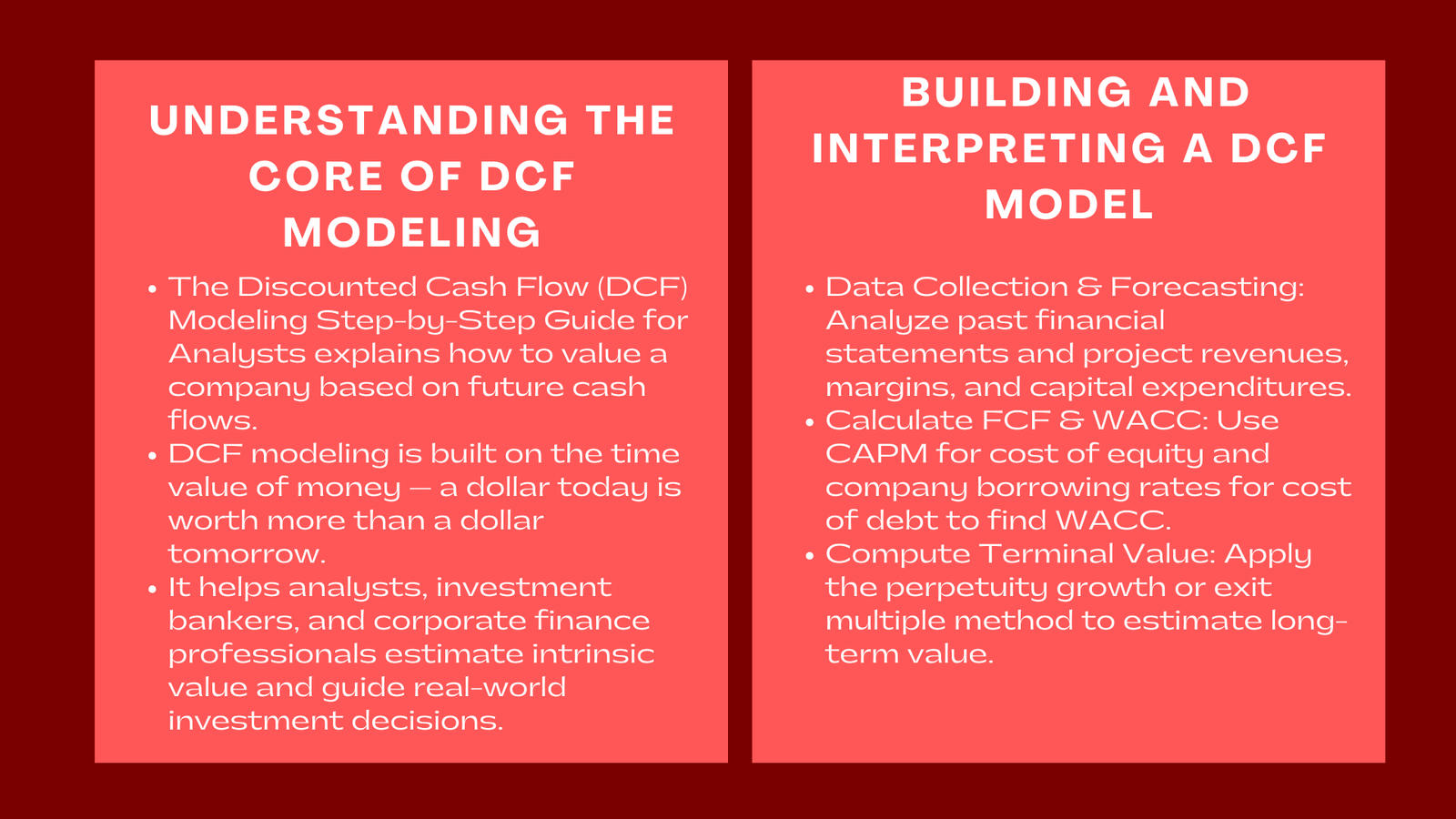
Before we get into the process of building a DCF, firstly analysts need to understand the thought process behind creating a DCF model. The approach is based on the principle of time value of money – it refers to the fact that a dollar today is worth more than a dollar in the future because of its possible earning ability. To reduce all of that to a numeric value, to determine how much a company is worth today, we take the free cash flows of that company in the future, and discount those cash flows back to today using a figure that incorporates both the riskiness of the cash flows and the time-investor’s rate of return.
The model known as DCF, refers to three major sections: forecasting free cash flows (FCF), identifying the discount rate (calculated more often than not as the Weighted Average Cost of Capital or simply WACC), and calculating terminal value to account for cash flows beyond the forecast period. Together these components provide the enterprise value of the business, or what we value the company as and we get the value of equity by subtracting the net debt and other adjustments.
Forecasting free cash flows is the most subjective and the most vital element of the DCF process. Analysts normally prepare projections of financial statements (income statement, balance sheet, and cash flow statement) for five to ten years into the future. The goal is to estimate the amount of cash that the business will generate after deducting its operating expenses, taxes, capital expenditures and any change in working capital. This measure, free cash flow to the firm (FCFF), is the amount of money available to the investors, both debt and equity holders. Professionals who attend a financial modeling and valuation training course in Singapore can learn how to perform such forecasting techniques accurately, ensuring realistic projections and sound investment analysis.
The second step is to choose a suitable discount rate. The WACC is the average rate of return needed by all providers of capital, weighted according to their percentage contribution to capital structure in the company. The cost of equity is estimated generally using the Capital Asset Pricing Model (CAPM) which takes into consideration the following: Risk-free rate of return, Beta (a measure of volatility in the equity market) of the company and the Equity risk premium. The cost of debt comes from borrowing rates of the company adjusted for tax deduction. Selecting correct inputs is important since minor variations in the discount rates may make a big difference in valuation results.
Finally, as it would be impractical to forecast the cash flows indefinitely, the analysts compute a terminal value in order to estimate the worth of the company beyond the projection period. This terminal value can be calculated through either the perpetuity growth approach (assuming that the cash flows increase at a constant rate indefinitely) or the exit multiple approach (which relies on the valuation multiple (such as EV/EBITDA) being applied to the financial metric of the final year). The present value of the terminal value plus the discounted cash flows will give the total enterprise value.
Step-by-Step Guide to Building a DCF Model
A well-structured logical progression must be taken to build a DCF model from scratch using Excel. It begins with collecting financial data and making assumptions based on past performance as well as expectations about the future. Analysts usually start by importing past financial statements and finding key ratios such as revenue growth, operating margins and reinvestment rates. It is these metrics that are used as a basis when forecasting future performance, which is also an essential foundation for buy-side and sell-side M&A valuation Singapore where precise financial modeling supports strategic investment decisions.
After the trends for history are determined, the analyst constructs the forecast section. Revenues are forecasted on the basis of growth assumptions based on industry trends, competitive position, and management guidance. Operating expenses are related to revenue drivers to ensure their consistency and operating margins are changed to account for anticipated efficiency gains or cost pressures. Depreciation and capital spending are linked to the asset base of the company and ensures that the reinvestment requirements are captured accordingly. The result is a projection of EBIT (Earnings Before Interest and Taxes) from which the taxes are taken to leave Net Operating Profit After Taxes (NOPAT).
The next stage is computation of free cash flow to the firm. Starting from NOPAT, analysts make non-cash additions such as depreciation and amortization, and minus capital expenditures as well as working capital changes. This gives annual free cash flow – the most important output of operational forecast. Each cash flow is the amount of money that that business generates which is available to distribute to investors, or to reinvest in the business.
With cash flows projected, the WACC is calculated by the analyst. Cost of equity estimated using the CAPM is given by:
Cost of Equity = Risk Free rate + Beta * Equity Risk Premium.
The cost of debt is the sum paid on interest rates to the borrowings of the company, after considering the benefit of tax shielding. The capital structure weights are based on the debt and equity market value. Combining these inputs gives us the WACC that is used to discount future cash flows to their current value.
The terminal value is then calculated, which represents often a rather big part of the total valuation of the company. The formula under the method of perpetuity growth is:
Terminal Value = Final Year FCF* (1 + g)/ (WACC – g):
where g denotes the long run rate of growth which is usually co-movable with economy (GDP or inflation expectations). Under the exit multiple method, the terminal value is calculated using a valuation value (e.g. EV/EBITDA) based on comparable companies or precedent transactions.
Once the analyst has determined the terminal value, the analyst discounts the terminal value and every forecasted free cash flow to present value terms using the WACC. The sum of these present values equal to the enterprise value of the firm. By subtracting the net debt, minority interests and other obligations, along with adding non-operating assets like cash the analyst reaches the value of equity. Dividing this number by the amount of outstanding shares gives the implied share price, which can then be compared to market price in order to determine if the stock is undervalued or overvalued.
Interpreting DCF Results and Applying Sensitivity Analysis
The interpretation of a DCF model extends beyond obtaining a single number. Risk management demands that analysts weigh up assumptions in credibility and the stability of the results in alternative situations. And because DCF valuations are so sensitive to inputs – certainly discount rate and terminal growth rate – even small adjustments can result in big differences in valuation. This is why sensitivity analysis is a part of any and every DCF model.
Analysts generally try to see what changes in key variables, such as revenue growth, WACC or terminal multiple – changes in such variables will impact the implied valuation. By developing sensitivity tables, they can graphically see how the results of valuation change for various combinations of assumptions. For instance, the WACC that is higher by 1% may decrease the enterprise value by 10% or higher, which shows the effect of perceived risk on valuation. Scenario analysis also provides this process with enhanced capabilities by allowing for the simulation of different business environments; base case, upside case or downside case, to account for the possible variability in performance.
A well-constructed DCF model should also make sense in line with other modes of valuation. While DCF is excellent in theory it is based on coming up with projections and assumptions that can be subjective. Therefore, often to ensure reasonableness, analysts tend to make comparisons between DCF results and valuations based on comparable company analysis (CCA) or precedent transactions analysis (PTA). If the result obtained from the DCF is far from market-based approaches, it may indicate that assumptions should be re-evaluated or justified with better evidence.
DCF modeling in real-life decision-making when making investment decisions, it helps to understand that there is a systematic way of valuation that helps us cut through the prize of noise in the market. For instance, in volatile equity markets where sentiments affect the prices up or down, a DCF valuation grounds analysis to the basic cash flow potential. Similarly, in the realm of project finance or capital budgeting, DCF analysis will help managers to determine whether the expected gain or returns exceed the cost of capital – an important factor in determining the creation of shareholder value.
Professional Relevance and Analytical Mastery
To financial analysts, the ability to create and decipher a DCF model is more than just a technical skill – it is a professional requirement. In investment banking, DCF models are used to support fairness opinions, valuations of acquisition targets and initial public offerings. In the private equity domain, they are used as tools for the valuation of acquisition targets or the projection of returns to the investor. In corporate finance, they provide decisions on capital expenditures, financing and strategic planning. Understanding DCF modeling puts analysts in the analytical position of disclosing the decision’s long-term impact, enabling a stakeholder to communicate results confidently.
Moreover, DCF modeling develops the way of thinking of an investor. It educates analysts to think about businesses, not as numbers on a spreadsheet, but as dynamic businesses with operating cycles and growth drivers, and competing issues. Through forecasting, analysts learn to assess strategic initiatives (such as entering new markets, as an example, or launching a new product or reorganizing operations) in terms of the impact on future cash flows and value to shareholders.
From a career perspective, the ability to use DCF modeling is often a prerequisite for promoting a career in finance. During recruitment processes candidates are often tested on their ability to explain the principles of DCF, justify assumptions and interpret outcomes. Employers find value in DCF competency as structured thinking, attention to detail and economic intuition. In addition to its importance in valuing companies, DCF modeling can be used to reinforce analytical foundations that can extend to other forms of financial modeling such as leveraged buyouts (LBO), mergers and acquisitions (M&A) and in project finance.
Conclusion
The Discounted Cash Flow model is still considered one of the most rigorous and insightful models in financial analysis. By concentrating on basic cash flow production and the time worth of cash, it overlooks brief-term market changes to provide the tremendous element of a business or investment. For analysts, the process of the DCF wanting to get up means the development of both technical precision and strategic understanding – the ability to forecast realistically, take on risk, and explain value with clarity.
Creating a DCF model is more than just learning the mechanics of valuation, it is about learning how to think. Each assumption represents a narrative about the future, each projection indicates a hypothesis about the performance of the business, and each discount rate represents a judgment on risk. The DCF model converts these elements into a logic internalized story of the value creation. In a profession where credibility is being measured by depth of analysis, the ability to construct, explain and defend a DCF model is still one of the best demonstrations of financial knowledge.